Prerequisites. Algebra up to quadratic equations and basic calculus. The proof in Section 3 uses a little real analysis, but you can skip it and still follow the main ideas.
1. What is training dynamics about?
One idea gaining traction in efforts to build a science of AI is to study how models change as they learn (i.e., their training dynamics). Recent papers make this case explicitly: Position: Don’t Just “Fix it in Post”: A Science of AI Must Study Training Dynamics from ICML 2026 argues that understanding model behaviour requires studying the training processes that produce it, while There Will Be a Scientific Theory of Deep Learning outlines an emerging “mechanics” of learning, built around quantitative predictions of how neural networks evolve during training.
So what is training dynamics? Broadly, it is the study of how a model’s parameters, representations, and predictions evolve during training, and how that evolution depends on the data, architecture, and learning algorithm. A useful formulation, in my opinion, comes from Ren and Sutherland’s (2025) Learning Dynamics of LLM Finetuning, which received an Outstanding Paper Award at ICLR 2025. In particular, they frame training dynamics as studying:
Change in parameters
Change in predictions
To study training dynamics, we first introduce gradient descent, the algorithm underlying many widely used methods for training neural networks. We measure how well a network fits the training data using an objective function, often called the loss function. A lower loss indicates a better fit, and the goal of gradient descent is to minimise it.
Ideally, we would find the minimiser analytically, much as we solve familiar calculus problems about maximising an area or minimising a volume. For neural networks, however, the objective is generally too complex to solve this way. Instead, gradient descent improves the parameters through a sequence of small updates, as shown in the pseudocode below.
Gradient descent
The block below is a “for loop”: it runs the instructions inside it sequentially, one line at a time, before starting the next repetition. Here, it calculates the gradient and then updates the weights, repeating this sequence \(K\) times in total.
\(\theta\) weights\(g\) gradient\(\eta\) learning rate
As seen in the pseudocode above, at each step of the loop, gradient descent updates the network’s weights \(\theta_k\) by moving in the direction opposite to the gradient of the training loss, \(\nabla L_{\mathcal{D}}(\theta_k)\). The learning rate \(\eta\) controls the step size:
You can think of the neural network’s objective function \(L_{\mathcal{D}}(\theta)\) as a landscape. The negative gradient points in the direction of steepest descent. Gradient descent takes a small step in that direction, recalculates the gradient at the new position, and repeats. This is very much like a ball rolling down a hill.
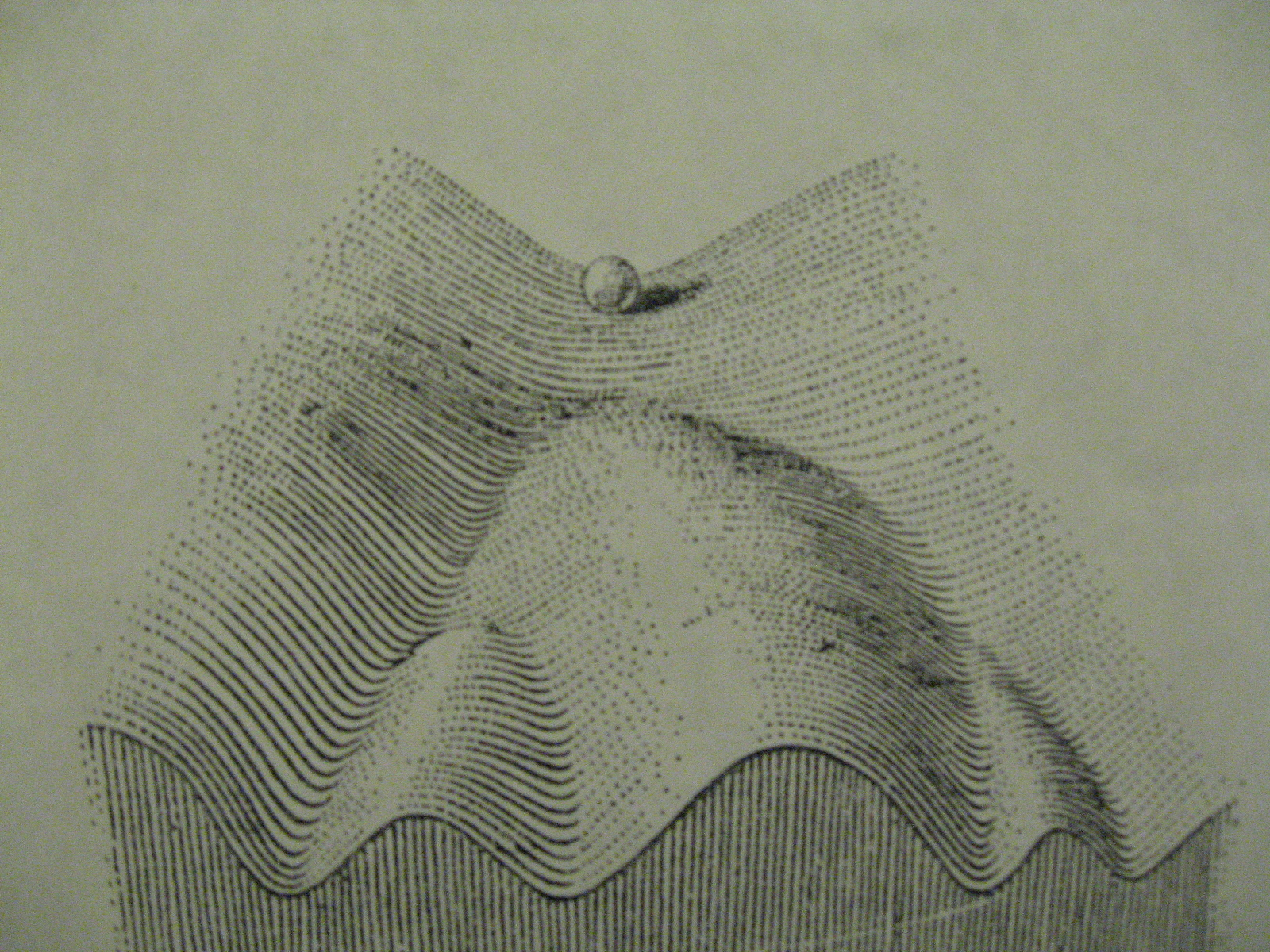
To take the analogy further, let us interpret each update as a step forward in time, with each step lasting \(\eta\). Defining \(t = k\eta\) and taking the limit as \(\eta \to 0\), the discrete updates approach a continuous trajectory governed by the differential equation below. This equation even resembles the equation of motion describing a ball descending into a valley under strong friction.
Gradient descent (continuous-time limit)
\[\frac{d\class{analogy-state}{\theta}}{d\class{analogy-time}{t}} =-\nabla\class{analogy-landscape}{L_{\mathcal{D}}}(\class{analogy-state}{\theta})\]Ball moving downhill (strong friction)
\[\frac{d\class{analogy-state}{\mathbf{r}}}{d\class{analogy-time}{t}} =-\nabla\class{analogy-landscape}{V}(\class{analogy-state}{\mathbf{r}})\]Show derivation: from Newton’s law to an equation of motion
1. Include the driving force and friction. Let \(\tau\) denote physical time. A ball of mass \(m\), moving in a potential \(V\) with a constant friction coefficient \(\gamma>0\), obeys
2. Neglect inertia when friction dominates. After the initial velocity has relaxed, assume the acceleration term is small compared with friction. The forces then approximately balance:
3. Rescale time. Define \(t=\tau/\gamma\). By the chain rule,
where the last equality uses the idealised model with inertia neglected.
This continuous-time description of gradient descent is called gradient flow. Throughout this introductory taster, gradient flow will serve as our “Mickey Mouse” model of the training algorithm.
2. Even yo mama can solve this neural network equation
Gradient flow alone does not make a neural network’s training dynamics easy to understand with pen and paper, so we will simplify the network too. Throughout these notes, we will consider a network with just two layers, one hidden unit, and no nonlinear activation:
The two scalar weights, \(a\) and \(b\), are all we train. Our goal is to learn the identity function \(y=x\), using fixed training inputs \(x_1,\ldots,x_n\), with at least one nonzero input.
These give us the training dataset \(\mathcal{D}=\{(x_i,y_i)\}_{i=1}^{n}\), with \(y_i=x_i\). For our learning problem, we define the objective function as the average squared prediction error, with a factor of \(\tfrac12\) to simplify its derivatives:
Here, \(n\) is the number of training examples, and \(f_{\theta}(x)=abx\) is the network’s prediction. The subscript \(\mathcal{D}\) reminds us which dataset we are fitting. Substituting our network and targets gives
Without loss of generality, we shall assume \(\frac1n\sum_{i=1}^{n}x_i^2=1\). This factor is a positive constant during training, so absorbing it into the time scale (or the learning rate for discrete updates) changes neither the solutions nor the training trajectory after that rescaling. We therefore use \(L_{\mathcal{D}}(a,b)=\tfrac12(ab-1)^2\) below.
Applying gradient descent to this loss gives the simultaneous updates
This problem is simple enough to solve without gradient descent. Since a square is non-negative, the smallest possible loss is zero, attained whenever \(ab=1\). Every pair of weights \((a,b)\) satisfying this equation is therefore a global minimiser of \(L_{\mathcal{D}}\).
Despite its simplicity, this model illustrates several results from the neural-network literature and helps us reason through some of the more surprising aspects of how neural networks learn.
For example, the objective \(L_{\mathcal{D}}\) gives us no reason to prefer \((1,1)\) over \((2,\tfrac12)\), or any other solution on the hyperbola \(ab=1\). When training reaches a zero-loss solution, what determines which one it finds? The preference among equally good solutions induced by the initialisation and the training algorithm (gradient flow in this case) is known as the implicit bias of training.
To understand this phenomenon of implicit bias, we begin with the following observation.
2.1. Key Observation: The network has rescaling symmetry
Consider multiplying one weight by \(\lambda\) and dividing the other by \(\lambda\):
The product \(ab\) does not change, so neither does the network’s output or its loss. In other words, we can increase the magnitude of one layer’s weight and compensate by decreasing the other’s, without changing the function the network computes. This simple symmetry has far-reaching consequences.
In particular, it implies a conservation law. The difference between the squared weights is conserved:
The weights can change, but this measure of their imbalance stays fixed at its initial value.
Show why rescaling symmetry gives a conserved quantity
Differentiating \(L_{\mathcal{D}}(\lambda a,b/\lambda)=L_{\mathcal{D}}(a,b)\) with respect to \(\lambda\) and evaluating at \(\lambda=1\) gives:
A connection to Noether’s theorem. Physicists often differentiate a continuous symmetry at the identity to expose its infinitesimal constraint—the starting move in many symmetry arguments, including the famous Noether’s theorem.
Under gradient flow, \(\dot a=-\partial L_{\mathcal{D}}/\partial a\) and \(\dot b=-\partial L_{\mathcal{D}}/\partial b\), so we get
Going deeper. The same argument applies to networks with nonlinear activations, provided the network retains this rescaling symmetry and the loss is differentiable with respect to the parameters. Under ordinary gradient flow without regularisation, differentiating the symmetry gives a conserved difference between the squared norms of the two groups of parameters being rescaled. Nonlinearity itself is no obstacle: the key ingredients are symmetry and differentiability. Kunin et al. (2021) study these connections between symmetry and conservation laws, and how practical training choices can break them.
The conservation law constrains the possible training trajectories. Starting from weights \((a_0,b_0)\), gradient flow stays on the curve
The only stationary points of \(L_{\mathcal{D}}\) lie on the zero-loss curve \(ab=1\) or at the origin. Combining this fact with the conservation law lets us determine the long-term outcome for each initialisation. The calculations below consider the cases \(c\ne0\) and \(c=0\).
Show the stationary points and training outcomes for both cases
If training starts with \(c=a_0^2-b_0^2\), its trajectory stays on the curve \(a^2-b^2=c\). Gradient flow is stationary wherever the gradient is zero; training generally approaches such a point as \(t\to\infty\). Any stationary endpoint must therefore satisfy
There are two possibilities. If \(ab-1=0\), both equations hold and the loss is zero. If \(ab-1\ne0\), the first equation forces \(b=0\) and the second forces \(a=0\). Thus the stationary points are
Case 1: \(c\ne0\). Conservation excludes the origin, since it has \(a^2-b^2=0\). Training reaches a zero-loss endpoint satisfying \(a_\infty b_\infty=1\) and \(a_\infty^2-b_\infty^2=c\). These determine its squared weights:
Calculating the zero-loss endpoint.
At zero loss, \(ab=1\), so \(a^2b^2=1\). Write \(u=a^2\); conservation gives \(b^2=u-c\). Substituting,
The quadratic formula gives \(u=(c\pm\sqrt{c^2+4})/2\). Since \(\sqrt{c^2+4}>|c|\), only the positive root can equal a squared weight. Thus
To check that training reaches this endpoint, use \(p=ab\):
For \(c\ne0\), the square-root factor is strictly positive. Thus \(p\) increases when \(p<1\) and decreases when \(p>1\), converging to \(p=1\).
If \(a_0>0\) and \(b_0>0\), both final weights take the positive square root:
Case 2: \(c=0\). Here the conserved set splits into two lines:
Gradient flow preserves each line. On \(a=b=s\), the dynamics reduce to
Every nonzero start approaches \(s=1\) or \(s=-1\), according to its sign, and reaches zero loss. On \(a=-b=s\), however,
Since \(1+s^2>0\), this always pushes \(s\) towards zero. Both weights approach the origin, where the loss is \(\tfrac12\). Starting at the origin itself leaves the network there.
Putting everything together, we can draw the diagram below. This is called a phase portrait: it shows the training trajectories and their long-term outcomes for our simple learning problem. The picture thus makes the implicit bias visible.
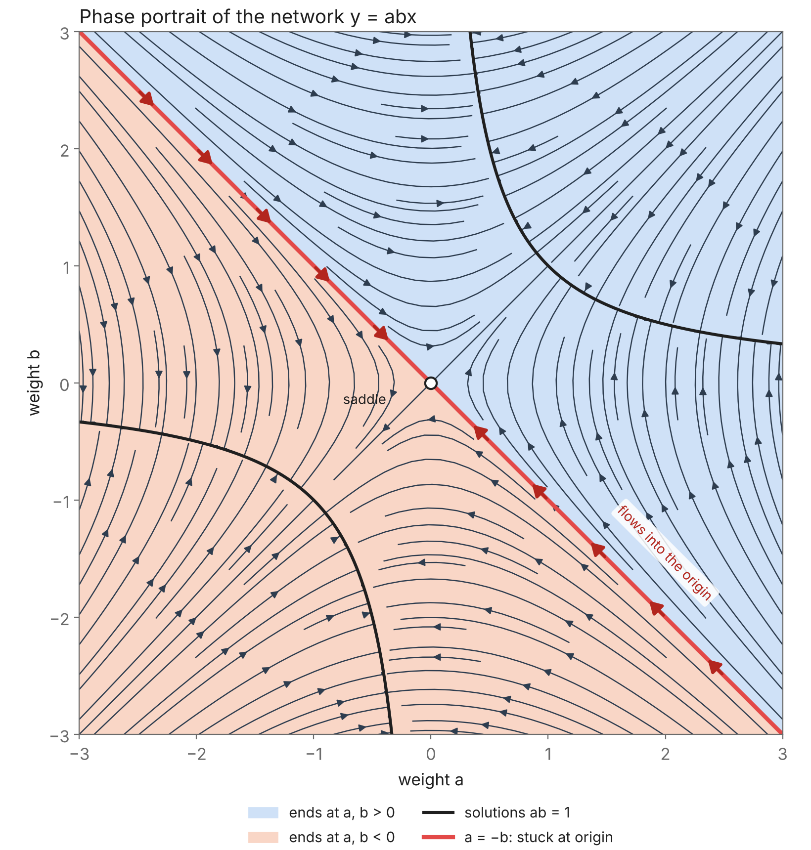
Each point in the diagram represents a pair of weights \((a,b)\). By choosing an initialisation and following the arrows, we can see how the gradient flow moves the weights, with each trajectory constrained by \(a^2-b^2=c\). The black curves mark \(ab=1\), where the loss is zero and training is stationary.
The colours show which branch training reaches. Initialisations in the blue region, where \(a_0+b_0>0\), converge to positive weights; those in the orange region, where \(a_0+b_0<0\), converge to negative weights. Both branches compute the same function, \(f(x)=x\). The red line \(a=-b\) separates these regions: its arrows lead towards the origin, where learning fails. A start arbitrarily close to this line, but not exactly on it, eventually reaches a zero-loss solution.
3. All models are wrong, but we can make them less wrong
3.1. How about finite step sizes?
With finite step sizes, the conservation law is broken. Writing the residual as \(r_t=a_tb_t-1\), the same calculation as above gives
To make matters worse, let’s consider the case where the step size is too large.
Choose \(\eta=1\) and \(a_0=b_0=2\). Then use pen and paper to compute the first few iterations:
We see here that the iterates diverge.
Thankfully, for any fixed initialisation, a sufficiently small positive step size ensures that the weights converge. Unless \(a_0=-b_0\), we can even show that they converge to a global minimum. We can also derive rates describing how quickly they approach it. With finite steps, the imbalance is no longer necessarily conserved. However, for a sufficiently small step size, we can replace the conservation equality with an inequality: the magnitude of the imbalance either remains unchanged or decreases.
These results are striking because the objective is non-convex, yet the algorithm uses a constant learning rate. Many introductory convergence proofs assume convexity, and some also require diminishing step sizes, leaving the setting discussed here outside their scope. Non-convexity makes global guarantees harder to establish, but this example shows that they can still be within reach. A fuller discussion of non-convex optimisation deserves a post of its own.
Show the proof of convergence (warning: advanced)
1. Take small enough steps. Choose
This keeps the weights bounded and ensures that the residual \(r_t=a_tb_t-1\) never changes sign, with \(|\eta r_t|<\tfrac14\). The algebra establishing these bounds is tucked away below.
2. Look at the sum and difference. Adding and subtracting the two weight updates gives
Both multiplying factors are positive. Since \(r_t\) never changes sign, one of the two magnitudes grows while the other shrinks (unless already constant). Neither sum nor difference changes sign, and both stay bounded because the weights do. They therefore have limits by the monotone convergence theorem for sequences.
Each weight is half the sum or difference of these two convergent sequences, so the weights themselves converge. Call their limits \(A\) and \(B\).
3. Find where they can end. Taking limits in the updates gives
Thus either \(AB=1\), giving zero loss, or \(A=B=0\). If \(a_0+b_0\ne0\), the origin is ruled out: when \(r_0<0\), the magnitude of the sum never decreases; when \(r_0>0\), the product stays at least one. If \(r_0=0\), we already have zero loss.
So training converges to a zero-loss solution unless \(a_0=-b_0\). On that exceptional line, the weights remain opposite, making \(AB=1\) impossible, so they converge to the origin instead.
4. Conclusion and also please do your homework
In conclusion, studying the training dynamics of our simple toy model has taught us how to identify conservation laws, understand when they break, and uncover the implicit bias of training. These are small, tractable versions of phenomena that also arise in much larger neural networks. Understanding how such behaviour emerges from the interaction between data, model structure, and the optimisation algorithm is what training dynamics is about. I hope this example has sparked your imagination about what a simple model can reveal and given you a feel for how researchers study training dynamics.
Reading can take us only so far, though. The Tutorial invites you to test the ideas by extending the model: add a ReLU nonlinearity, introduce weight decay, add more layers, and explore how label noise interacts with weight decay. Working through these exercises lets you see which conclusions survive, which depend on our assumptions, and what new behaviour emerges, much as a researcher would.
If you are still not convinced, consider this. With weight decay, our toy model exhibits a phase transition, as seen in the diagram below.
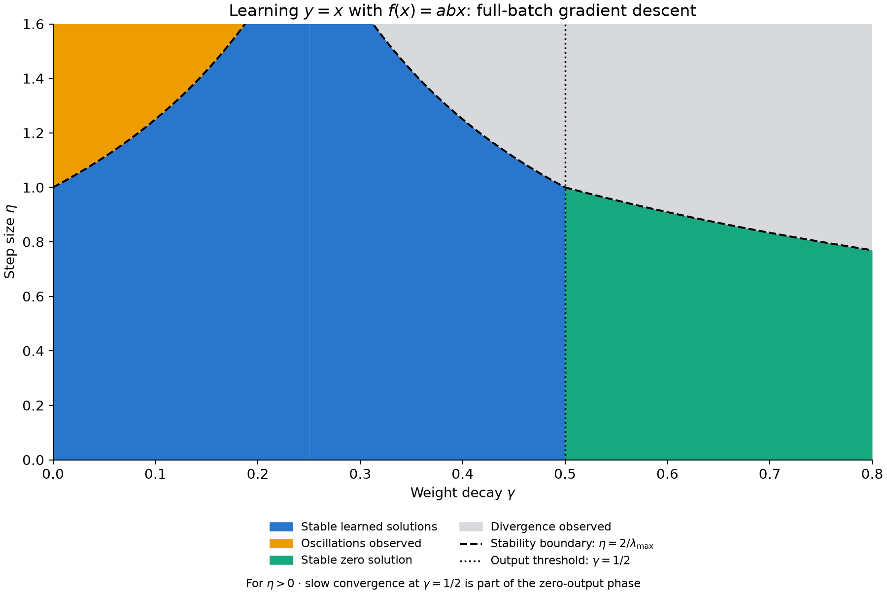
As the decay strength crosses a critical value, the learned output shrinks to zero and the network stops fitting \(y=x\). The decay strength plays a role rather like temperature in a material: changing one control parameter can change the system’s qualitative behaviour. At greater depth, the transition becomes even more striking. The tutorial leads you through both results. This is a glimpse of how much structure this small model contains. I hope you will find it a useful starting point for your own exploration of training dynamics. Till next time
Footnotes
1 GPT-OSS and DeepSeek-V4.1 clamp branch values, possibly for numerical stability. Fixed clipping thresholds on the rescaled branch break the exact symmetry; GPT-OSS also adds an offset. ↩
References
Biderman, S., Khan, M. A., Mireshghallah, N., Arnett, C., Barez, F., & Saphra, N. (2026). Position: Don’t just “fix it in post”: A science of AI must study training dynamics. In Proceedings of the 43rd International Conference on Machine Learning (Vol. 306, pp. 169526–169542). Proceedings of Machine Learning Research. https://proceedings.mlr.press/v306/biderman26a.html
Blanc, G., Gupta, N., Valiant, G., & Valiant, P. (2020). Implicit regularization for deep neural networks driven by an Ornstein-Uhlenbeck like process. In Proceedings of the Thirty Third Conference on Learning Theory (Vol. 125, pp. 483–513). Proceedings of Machine Learning Research. https://proceedings.mlr.press/v125/blanc20a.html
Cohen, J. M., Kaur, S., Li, Y., Kolter, J. Z., & Talwalkar, A. (2021). Gradient descent on neural networks typically occurs at the edge of stability. In International Conference on Learning Representations. https://openreview.net/forum?id=jh-rTtvkGeM
Damian, A., Ma, T., & Lee, J. D. (2021). Label noise SGD provably prefers flat global minimizers. In Advances in Neural Information Processing Systems, 34. Conference paper.
Kunin, D., Sagastuy-Brena, J., Ganguli, S., Yamins, D. L. K., & Tanaka, H. (2021). Neural mechanics: Symmetry and broken conservation laws in deep learning dynamics. In International Conference on Learning Representations. https://openreview.net/forum?id=q8qLAbQBupm
Ren, Y., & Sutherland, D. J. (2025). Learning dynamics of LLM finetuning. In International Conference on Learning Representations. Conference paper.
Saxe, A. M., McClelland, J. L., & Ganguli, S. (2014). Exact solutions to the nonlinear dynamics of learning in deep linear neural networks (arXiv:1312.6120). arXiv. Paper (PDF).
Simon, J., Kunin, D., Atanasov, A., Boix-Adserà, E., Bordelon, B., Cohen, J., Ghosh, N., Guth, F., Jacot, A., Kamb, M., Karkada, D., Michaud, E. J., Ottlik, B., & Turnbull, J. (2026). There will be a scientific theory of deep learning (arXiv:2604.21691). arXiv. https://arxiv.org/abs/2604.21691
Cite this taster
If this taster is useful in your work, you can cite it with this BibTeX entry.
@misc{ang2026learningdynamics,
  author = {Ang, James Ming Liang},
  title = {Training Dynamics},
  year = {2026},
  month = oct,
  note = {Science of Deep Learning: Taster Series},
  url = {https://jamesmldoesml.github.io/blogs/learning-dynamics/}
}